Variational Autoencoder

Compression of images into a vector representation. VAEs allow clustering of similar images in space. Can also randomly generate images. Maps the input space of images onto a very low dimensional space. For an analysis please see below!

About this Project

Here is a simple implementation of a VAE using tensorflow.

The parameters to be tuned can be accessed in params.py. Analysis below used these parameters.

The purpose of this repository is to learn and test an understanding of VAES. Please see the VAE background section, this will get us an understanding of VAEs, which we can then test. See the Analysis section for an analysis of the VAE.

Code is here

VAE background

Resources

These are great resources for VAEs:

Original Paper: Auto-Encoding Variational Bayes
Explanation: Tutorial on Variational Autoencoders

Theory

What is a latent space?

This is the representation defined by the bottleneck layer of the network. This representation is called the latent representation, which is used to generate the observable data, X.

The latent space is just the continuous set of all these latent representations.

How does VAEs construct a latent space?

Here is the problem: Train on a single point won’t give good results for the points around that point. If we were to just deterministically backprop the difference (as is what happens with a normal autoencoder), we might not get good results when sampling the parts of the space that aren’t training data representations.

To solve this, we should train a region around X for a given point X. Using the information in X to shape a region in space. Using many of these X will allow us to create our space. The region between two training points will be an interpolation between the two points.

Another desireable of our space is if we can cause a small region in our space to generate the desired data, as we get further from this region, generation of X becomes more unlikely. This will allow us to use the information within the data efficiently.

How do we implement this solution? We will have our latent representation be a distribution instead of a deterministic point or a dirac delta. When training, we can update the parameters in this distribution.

How do we choose a distribution? The standard distribution to choose would be the normal distribution (this is what the paper uses). No matter what the image distribution is (for a given X), our encoder neural network should be able to map the distribution to a normal, (this is our prior). See Figure 2 in Tutorial on Variational Autoencoders. We can represent the bottleneck layer as a distribution by calculating the mean and standard deviation.

Prevent the distribution from collapsing to a point! Even if we set up our network to be able to represent a probabilistic latent representation, there is nothing preventing the network from setting the standard deviation to zero. Nothing in our objective accounts for the space between training samples. We need to constrain our latent representation distribution. This is where the KL divergence regularization term comes in. We will constrain it be close to our prior. We try to minimize the KL divergence between the prior (which is an isotropic normal) an our calculated distribution. By doing this we have also forced the images generated to be anchored to the same distribution/region of space (centered around 0), which is what we also desired.

Implementation Tricks

reparameterization trick:

What is it?
- We won’t be able to backprop through a random variable. This means that we won’t be able to update the inference model, as our latent representation will be a random variable.
- The reparameterization trick aims to solve this by separating the deterministic part and the random part. We can have mean and standard deviation be deterministic, where we can back propogate through, and have a noise term which get mulitplied to the standard deviation, which will cause this to be random.
How to code it? We need to constrain our standard deviation to be positive, since our KL loss depends on that. We can either apply a softplus to the stddev, or we can allow it to be negative and say that the network is calculating the natural log of the stddev, which is what this project does.

Analysis:

AE vs VAE

To first test out our theory, lets look at the difference between an autoencoder and a Variational Auto Encoder.

It should be easy to switch between the two of them, if we were to just leave out the KL divergence term, we will only be fitting the training data, with dirac deltas, as we are setting X=f(X) (which defines a single point, X). This means that we can expect very good reconstruction, but very poor generation. VAEs will have equal, or worse reconstruction than this, as they are optimizing for a region in space. So, our VAE loss will be bounded by our AE loss. After a bit of testing, we can see that our AE loss is 0.004 (MSE).

Problem with the learned representations.

When converting our network from a AE to a VAE, we start to see a problem. The KLD loss becomes 0! This causes the posterior distribution to be equal to the prior, which will generate the same image every time!

Mean Squared Error and KL Loss

The loss for the reconstruction is being overshadowed by the KLD loss (regularization loss). We should then, increase the KLD loss slowly, give the reconstruction loss some time to re-adjust.

We put a weight parameter on the KLD term:

wait until model reached sufficent reconstruction quality, then increase the weight by a fraction at each step, cap at 1.

This problem called posterior collapse. The model makes predictions independent of the latent representation, and will therefore try to solely minimize the regularization term instead. This causes the posterior to become equal to our prior, all our training representations collapse down to the same distribution.

To solve this Bowman et al. mention in section 3.1 that they increase the KLD loss slowly from 0 to 1, called KLD annealing.

Section 2.2 of Chen et al. mention that posterior collapse is caused by an expressive decoder, where the decoder could sufficiently model x without z. They look at this using a bits-back approach.

Model Architecture

the architecture that I used for this loss training:

Encoder: 2x Conv Layers, [64,4,2], 1x fully connected layer [256]
Latent Space Size: 32
Decoder: 1x Conv Layer [64,4,2], 1x Conv Layer [1,4,2], 1x fully connected layer [256]

Additionally I used a batch size of 64

Autoencoder Analysis

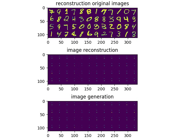
Let’s first analyze a VAE with the KLD weight set to 0, just as an initial test to see if our model can run on the data. We need to see if the model has the capacity to learn the data.

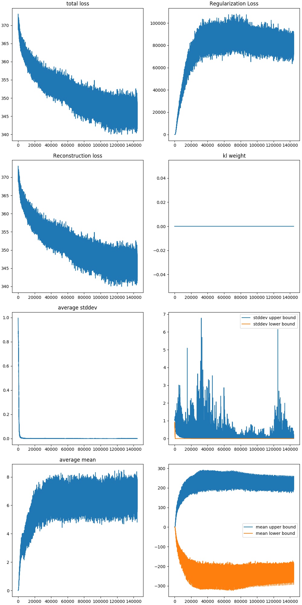
Autoencoder Training Samples. Smaller pixel values were increased, to make them more prominent. Autoencoder Training Values, The upper and lower bounds are the highest and lowest values in the test batch for their repective labels (ie. mean and stddev).

Here, we see that the theory above is correct. We see from how the images evolve, that the model is capable of learning the images. Notice how the standard deviation of the latent variables are being minimized to 0.

Since our model is not constrained, the goal of the model is to directly minimize the loss from the training samples, and thus has poor generation abilities. Mathematically, this is shown from the mean and standard deviation of the latent variables, which can be see as interpolations, or a bridge between the control points of the training samples. The model tries to minimize the effect each item has on one another, causing the increase in mean and the decrease in standard deviation.

KLD Annealing

Now, lets try KLD annealing mentioned before. We can slowly increase the regularization term weight, while letting the reconstruction catch up. The rate of increase will be done empirically (through experiments). We can start increasing the weight after a while of letting the reconstruction term learn in an AE manner first (weight=0), to get a foothold.

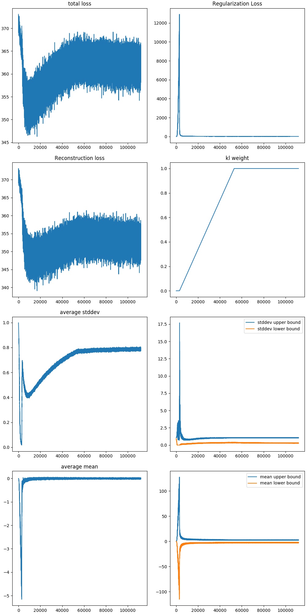
Autoencoder Training Samples with KLD Annealing. Smaller pixel values were increased, to make them more prominent.

Autoencoder Training Values with KLD Annealing, The upper and lower bounds are the highest and lowest values in the test batch for their repective labels (ie. mean and stddev).

Here we can see that the generation results are better, and the reconstruction results seem to be less grainy as well, which might be an effect of using information from other, similar training points. This might be an effect of compression, where good representations are being forced to be learned to minimize the space due to the constraint (regularization term). However, over training, it seems like the numbers are noiser, this is probably due to the effect of the increase in the standard deviation term, causing more noise to be added (it is not being minimized to 0 now.). We can see how much more constrained the distributions of the latent variables are now. The ranges for the mean is smaller, where as the standard deviations are larger now.

Decreasing Model Capacity

Another reason on why posterior collapse would happen is due to the decoder having high capacity. We can test this out by simply decreasing the capacity of the VAE.

Convolutional neural networks have the assumption of invariance to position built into the achitecture through the sliding window (kernel). This means that it won’t have to learn this quality of the data. Normal neural networks perform worse, since they need sufficient data and model capacity to be able to learn this feature. Therefore, we should be able to decrease model capacity by introducing a normal feed forward neural network as the encoder and decoder.

The architecture I used was:

a two 500 unit hidden layer feed forward neural net for the encoder with relu activations.
a one 500 unit hidden layer feed forward neural net for the decoder with relu activation.

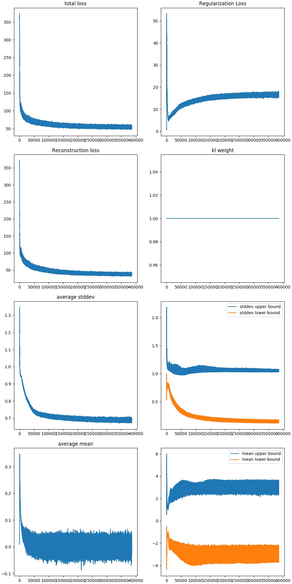
Variational Autoencoder Training Samples with low capacity. Smaller pixel values were increased, to make them more prominent.

Variarional Autoencoder Training Values with low capacity, The upper and lower bounds are the highest and lowest values in the test batch for their repective labels (ie. mean and stddev).

This method seems more stable. We see that in the beginning the images start to all look similar and the KLD loss is approaching 0, representative of mode collapse. However, after a bit of training, the model is able to regain good representations. This seems much more stable than a high capacity network.